CUTLASS CUTE 1 Layout Algebra
约 3940 个字 109 行代码 4 张图片 预计阅读时间 21 分钟

这是整个 cute 的核心,并且 cute 本身文档很难读,而且网上没有太多的学习资料,所以就算是 GPT 也很难给出好的回答。我的学习资料主要来源于三个部分:1. Reed zhihu 2. Lei Mao's blog 3. A note on the algebra of CuTe Layouts
我想以三个部分来介绍,目的是为了形成对 layout algebra 的清晰理解
- layout 基本概念
- layout algebra 基本运算
- layout algebra 组合运算
基本概念
layout 概念非常简单,就是由两部分组成:shape & stride,二者共同构建出一个整数到整数的映射:\(\mathbb{N} \rightarrow \mathbb{N}\)
为了完成这个映射,我还需要引入一个概念:整数与多维坐标的同构性 (isomorphism)。在数学上,两个东西同构意味着二者本质上是一个东西,二者可以通过一个映射进行可逆的转换。现在我们来构建整数与多维坐标的转换,就能够证明二者的同构性。我们定义多维坐标是 shape 空间中的一个点\((x_0,x_1,...,x_{n-1})\),通过点积我们就能完成多维坐标到整数的转换
而整数到多维坐标的转换则是通过取余完成
实际上这就是列优先的顺序排列方式
有了以上的转换过后就可以定义 layout function 映射了,定义为如下
其中\(f'(·)\)即为将整数转换为坐标的映射,而\(g(·)\)为将坐标转换为整数的映射,其本质是坐标 coord 与步长 stride 的点积
如此一来我们就完成了从整数到整数的映射:我们从整数\(x\)出发,寻找其对应的坐标点,然后通过步长进行新的映射
此时你可能发现了,将\(f\)与\(g\)其实非常相似,都是将坐标映射到整数。在之前我也提到了,\(f\)本身就是 column-major 的排列方式,其可用一个特殊的 layout 来表示,该 layout 我们称之为 layout left (or natural layout)
举一个例子,一个 shape 为 (2, 3) 的 natural layout 为
有了 layout left,那就有 layout right,也就是行主序排列
Layout 其中一个作用就是用来描述坐标与内存位置。这是很自然的事情,因为物理内存永远都是以一维的形式来表达,所以在 cutlass cute 中就是用一个指针 + 一个 layout 来描述一个 tensor,并且在 cutlass 中以 shape:stride 的形式 print layout
Tensor(Ptr const& ptr, Layout const& layout)
Layout(shape=[2, 3], stride=[3, 1]) // (2, 3):(3, 1)
而实际上 Layout 可以用来描述更多的事情,例如:如何将一个\((M,N)\)形状 tensor 分配到\((T,V)\)形状当中。其中\(T\)就是 threads 数量,\(V\)是每一个 thread 拥有的 values,这将在基本运算小节中进行介绍
基本运算
layout algebra 最抽象的部分在于其基本运算,尤其是以下两个基本运算:
- complement,补运算
- compose,复合运算
当然还有其他的运算,例如 concat, coalecse,我用代码来简单解释
"""
@dataclass
class Layout:
    shape: List[int]
    stride: List[int]
"""

A = Layout([2, 3], [1, 2])
B = Layout([4], [10])
coalesce(A) # Layout(shape=[6], stride=[1])
concat(A, B)# Layout(shape=[2, 3, 4], stride=[1, 2, 10])
concat 就是将 shape & stride 分别连接,而 coalecse 则是合并 shape & stride,以更少维度呈现
Complement
补运算需要两个元素,整数\(M\)和 layout 本身。我先用一个一维的例子来说明补运算的作用,这也是 reed zhihu 中所使用到的例子
在 reed zhihu 中说到
当codomain存在不连续时,则存在空洞的位置,如图4所示,这时候我们可以构造一个Layout2能够填充上codomain的空洞位置,此时我们构造的Layout则为原Layout的补集
我认为 complement 的作用是计算出了 layout 所需要重复的“次数”以填满整个\(M\)空间。用上面的例子来说
A 还需要重复两次才能够填满 0~8 的整个空间,而后面的 stride 则描述了重复空间之间的间隔,在这里间隔是 1。实际上只需要将 A 和 A 的补 concat 起来就会发现,二者组成了一个连续的空间
在这个 case 中 concat 过后的结果是一个 layout right 排布
再举一个二维的例子
A = Layout([2, 3], [2, 4])
B = complement(24, A)   # Layout(shape=[2, 2], stride=[1, 12])

# Layout A
#     0      4      8
#     2      6     10

# Layout([4, 6], [1, 4])
#     0      4      8     12     16     20
#     1      5      9     13     17     21
#     2      6     10     14     18     22
#     3      7     11     15     19     23
可以看到 A 需要在两个维度(在 cutlass 中习惯把一个维度称之为一个 mode)的方向上都分别重复两次。在第一个 mode 上重复空间的间隔是 1,而在第二个 mode 重复空间的间隔是 12。我们仍然可以将 A 和 B 进行对应 mode 的 concat
A = Layout([2, 3], [2, 4])
B = Layout([2, 2], [1, 12])
C = Layout([(2, 2), (3, 2)], [(2, 1), (4, 12)])
concat 之后的 Layout C 实际上可以看做一个合并的 Layout([4, 6], [1, 4])
现在我们再来看 complement 的公式就会发现其中的奥秘:
其本质就是在计算每一个 mode 还需要重复多少次才能够填满整个空间,重复空间的间隔即为子空间大小\(s_id_i\)
Compose
既然是映射(函数),那么将两个函数进行复合是再正常不过的想法了。从直观上来说将两个 layout 进行 compose 非常简单,毕竟都是整数到整数的映射:
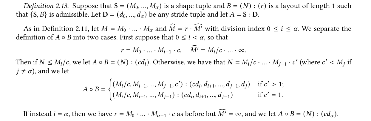
但是需要考虑的问题是,如何将新的 compose 结果\(g_3\)描述为一个合法的 layout 结构 (shape, stride)。而这个描述其实还是要化不少笔墨介绍的,这里省略,可参考 Definition 2.13 from A note on the algebra of CuTe Layouts
NOTE: 其实 layout algebra 对于输入其实都是有要求的,并不是任意两个 layout 进行 compose 都是可行的,其对于整除性还是有不少要求。好消息是如果数值都是以\(2^n\)存在,整除性质就会得到很好的保障,而这正是在 GPU 编程中常用的数值。
虽然说需要严谨的数学来保证 compose admissibility,但这不妨碍其本质就是上述所说的复合函数,即:从一个 domain 映射到另一个 domain。我将以一个非常具体的例子帮助理解这个 compose 过程
首先我定义了两个 layout,第一个 TV2MN 描述了 thread values 所对应的 MN 映射。第二个 MN2Memory 描述了 MN 到内存的映射。更具体来说
TV2MN描述了 4 个线程,每一个线程拥有有 (2, 2) 个 values,这些 values 将映射到一个 shape 为 (M, N) 的 tensor 上。该 layout 也将描述 tensor 是如何被分配到线程当中的MN2Memory描述了 tensor 中各个坐标的 value 在内存当中的位置。在例子当中是一个 layout right 的排布,也就 tensor 在内存中是行优先排列
通过 compose 我们可以直接获得 TV2Memory 这样的映射,该映射即代表了内存中的数据如何被分配到线程当中
我们将这个例子打印出来,通过 step by step 的方式看下整个 compose 的过程:
TV2MN: Layout(shape=[4, 2, 2], stride=[2, 1, 8])
        0|     1|     8|     9|
        2      3     10     11
        4      5     12     13
        6      7     14     15
MN natural: Layout(shape=[4, 4], stride=[1, 4])
        0|     4      8|    12
        1|     5      9|    13
        2      6     10     14
        3      7     11     15
MN2Memory: Layout(shape=[4, 4], stride=[4, 1])
        0|     1      2|     3
        4|     5      6|     7
        8      9     10     11
    12     13     14     15
TV2Memory: Layout(shape=[2, 2, 2, 2], stride=[8, 1, 4, 2])
        0|     4|     2|     6|
        8     12     10     14
        1      5      3      7
        9     13     11     15
以 thread 0 为例:
- 其对应的 MN index 为
(0, 1, 8, 9) - 通过 MN index 可以找到
(0, 1, 8, 9)分别对应坐标(0,0), (1,0), (0,2), (1,2) - 通过对应坐标找到
MN2Memory所对应的值为(0, 4, 2, 6) - 所以 thread 0 的 4 个 values 将会寻找内存中第 0, 4, 2, 6 个元素
由此我们就完成了一个映射,其从 TV domain 出发,映射到了 Memory domain。这也引出了 compose 的一个直观性质:不改变 source domain,即输入的 layout “形状”是不会改变的
TV2MN: Layout(shape=[4, 2, 2], stride=[2, 1, 8])
TV2Memory: Layout(shape=[(2, 2) 2, 2], stride=[8, 1, 4, 2])
Inverse
同样的,在函数中也存在逆函数。在 layout algebra 中的逆函数定义可参考 reed-zhihu 中的 two line notation 表示形式。所谓的 two line 就是:input domain 为一个 line,output domain 为一个 line,下面举一个例子
# Layout(shape=[2, 3], stride=[3, 1])
# [0, 1, 2]
# [3, 4, 5]

coord: [0, 1, 2, 3, 4, 5]
value: [0, 3, 1, 4, 2, 5]

# sort the pair according to value
coord: [0, 2, 4, 1, 3, 5]
value: [0, 1, 2, 3, 4, 5]

# switch coord and value as new layout
coord: [0, 1, 2, 3, 4, 5]
value: [0, 2, 4, 1, 3, 5]
上述 two line notation 用于理解 inverse 是比较直观的,但是对于理解 inverse 过后 layout 形式是怎么样的,没有太大帮助。具体来说,他们的 shape & stride 应该如何得到?在 Lei Mao's blog 当中证明了 compact layout inverse 过后的 shape & stride 应当如何计算,不过 blog 当中的叙述顺序对我来说略显晦涩,我这里用我自己的思考逻辑来整理
Conditions:
-
Layout function:\(f_L(x)\)
-
shape & stride 为\(S=(s_0,s_1,...,s_n),D=(d_0,d_1,...d_n)\)
-
natural layout funciton 将多维坐标\((x_0, x_1, ...,x_n)\)映射为\(x\)
\[ x=x_0+x_1·s_0+...+x_n·\prod_0^{n-1}s_i \]
Target:
-
找到 inverse layout:\(f_{L'}(x)\)使得满足
\[ f_{L'}(f_L(x)) = x \] -
inverse layout\(L'\)shape & stride 为\(S'=(s_0',s_1',...,s_n'),D'=(d_0',d_1',...d_n')\)
现在开始正式推导。对于输入\(x\)对应的\(L\)坐标为\((x_0, x_1, ..., x_n)\),我们设其输出为\(x'\)
输出\(x'\)所对应的\(L^{-1}\)坐标为\((x_1',x_2',...,x_n')\),由\(L'\)shape 的 natural layout function 完成映射。由等式条件得
其中最重要的等式为
下面的证明思路为:如果我们能够找到一个 permutation\(I=\{i_0,i_1,...,i_n\}\),使得\(x_{i_0}'=x_0,x_{i_1}'=x_1,...,x_{i_n}'=x_n\),那么我们就能对应多项式的每一项,直接算出每一个\(d'\)的值。现在我们来考察\((x_0,x_1,...,x_n)\)与\((x_0',x_1',...,x_n')\)之前的联系是什么,是否存在这样的 permutation
他们之间的关系非常清晰
这里的\(N\)就是 inverse layout 的 natural function。现在问题转换为:对于一组\((x_0,x_1,...,x_n)\)与\((x_0',x_1',...,x_n')\),他们彼此都是对方的 permutation,我们需要找到合适的 natural layout function 即可。其实对于第一个要求非常好满足(忽略 natural layout 限制),我们可以直接对\(L\)中的 shape & stride 进行 permute 即可。以简单的 Layout(shape=[2,3], stride=[3,1]) 为例子,当 permute shape & stride 时,坐标也随之 permute
现在只需要考虑 natural layout 的限制即可,而答案也就随之浮出水面:只需要将\(L\)的 shape & stride permute 成为一个 natural layout (left layout) 即可。更具体来说,根据 stride 的大小,从小到大进行排列,由于 layout 有 compact 保证,没有任何空洞,所以排列出来的 layout 必定也是 natural layout。所以此 permutation 存在且唯一,确定了 inverse layout 的 shape,其对应的 stride 也可由下面的式子进行计算
那么根据上述结论,我们就找到了\(L'\)的 shape & stride 了!其中 shape 的结论会很 clean,就是将\(L\)进行 sort 过后的 shape。从定性来说:原始 stride 小的 shape 在 inverse 过后会靠前;反之则会靠后
而在 写给大家看的 CuTe 教程:Layout compose & Inverse 中提到,通常 inverse 过后还会使用 with_shape 来构建我们期望的 layout shape,我们必须要了解 inverse 的输出形状到底是什么,才能正确地使用 with_shape。具体的例子在 retile 部分中,计算 (t, v) -> (m, n) layout 进行展示,其精妙地展示了 inverse 的一个核心作用:domain 的交换。如果我们获得了 (m, n) -> (t, v) 的映射,直接使用 inverse 就可以获得 (t, v) -> (m, n) 映射
组合运算
有了 layout algebra 所定义的基础运算就可以定义一些更复杂更有用的运算:divide & product
divide
divide 是划分数据中最常用的方法,尤其是 zipped divide。我先介绍 logical divide 的一维运算公式(B 是维度为1的 layout,A 没有限制)
def logical_divide(A, B):
    M = A.size()
    c_B = complement(M, B)
    concatenated = concat(B, c_B)
    return compose(A, concatenated)
可以看到,其先计算了 B 补集,然后与 B 进行了 concat,最后用 concat 过后的 layout 与 A 进行了 compose。通常我们称 layout B 就是一个 Tiler,以 Tiler 为粒度对 A 进行了划分。在实际应用过程中都是对一个 layout 进行逐维度 divide (by-mode divide)
Layout Shape : (M, N, L, ...)
Tiler Shape  : <TileM, TileN>

logical_divide : ((TileM,RestM), (TileN,RestN), L, ...)
zipped_divide  : ((TileM,TileN), (RestM,RestN,L,...))
在上面的例子中 Tiler 是不连续的,而我们更常会遇到的 Tiler 是最简单的 stride 为 1 的 Tiler。如 B = Layout([4], [1]),这样就会以 4 为单位切分该轴。zipped divide 会将 Tiler 维度直接提到最前面来,以方便我们进行索引操作,通常这个维度可以是 thread,这样通过索引就获得具体某个线程所对应的数据
通常我们遇到的情况都是:A & B 都是 1-dim,如果 A 为多维 layout,那么就需要谨慎看待,最后的结果一般不是我们想要的。举个例子
l1 = Layout([5, 4], [1, 30])
l2 = Layout([4], [1])
# logical_divide(l1, l2) won't work
A size: 20
complement of B: Layout(shape=[5], stride=[4])
concated (B, c_B): Layout(shape=[4, 5], stride=[1, 4])
原因在于 concated layout 无法和 A 进行 compose。不过好消息是在进行数据 divide 时,通常是对 MN shape 进行 divide,这是一个非常规整的 domain,满足我们在 by-mode divide 时各个 mode dim 都是 1 的需求
product
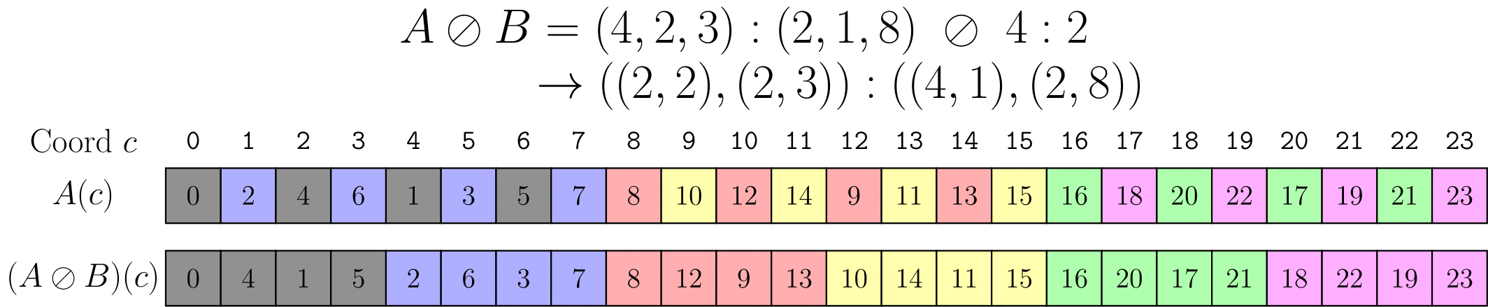
这里有个割裂感:我们说 product 为 divide 的逆运算,但实际上我发现二者并不能进行可逆操作。例如 C != A.product(B).div(B)。但是这个定义并不符合我们的直觉,严谨的数学定义在 Lei Mao's blog 中有所阐述。这里以一个 2D exmaple 作为说明
这个 product 的结果非常直观:把 (2, 5): (5, 1) 进行重复,重复维度为 (3, 4)。在我的期望中,直接使用 tiler <3:1, 4:1> 就能完成上述功能,但实际上用的 tiler 为 <3:5, 4:6>,这就是因为 product 的定义并不是我们想象中的直观,仍然是根据 complement & compose 来定义的。为了让 product 功能与我们的编程直觉相符,cute 直接构建了几种常见的 api 方便调用,参考 reed zhihu
| 乘法模式 | 乘积的shape |
|---|---|
| logical | ((x, y), (z, w)) |
| zipped | ((x, y), (z, w)) |
| tiled | ((x, y), z, w) |
| blocked | ((x, z), (y, w)) |
| raked | ((z, x), (w, y)) |
上面只列举了 shape,对于 stride 而言,相同 dimension 的 stride 也是一样的:即任意乘法模式中所有 x 对应的 stride 都一样。需要注意的是,这些操作是 layout x layout,而不是 layout x tiler。所以他们都是 rank sensitive 的,即两个 layout 的维度必须一致。同时和 divide 一样,通常使用在相对规整的 domain,即 layout 的 size 和 cosize 一致。否则存在空洞的话,product 也可能无法进行,举一个例子
auto l1 = make_layout(make_shape(_4{}, _5{}), make_stride(Int<30>{}, _1{}));
auto l2 = make_layout(make_shape(_2{}, _4{}));
// can't do logical_product(l1, l2)
这里点出一个 product 和 divide 的重要差异:divide 习惯使用 layout divide tiler,而 product 习惯使用 layout product layout。另外一个实验是,product 的顺序是会改变结果的
auto base_layout = make_layout(make_shape(_4{}, _3{}), make_stride(_4{}, _1{}));
auto layout_x2 = blocked_product(base_layout, make_layout(make_shape(_1{}, _2{})));
auto layout_x2_x2 = blocked_product(layout_x2, make_layout(make_shape(_2{}, _1{})));
auto layout_x4 = blocked_product(base_layout, make_layout(make_shape(_2{}, _2{})));

// Product order test
// ((_4,_1),(_3,_2)):((_4,_0),(_1,_16))
// (((_4,_1),_2),((_3,_2),_1)):(((_4,_0),_32),((_1,_16),_0))
// ((_4,_2),(_3,_2)):((_4,_16),(_1,_32))
我先对 base layout 在第二个 dim 进行扩张,然后再对第一个维度进行扩张,其结果和同时扩张两个维度是不一致的。在之后的内容当中,我们可以使用组合运算和基础运算来获得所需的 layout 排布,在实践中学习