CUTLASS CUTE 8 hpc-ops 之 group gemm 实现细节
约 3395 个字 219 行代码 2 张图片 预计阅读时间 20 分钟

本篇博客整理了三个 hpc-ops 在 group gemm 当中的实现细节作为上一篇博客的补充:
- Transposed MMA — 小 M 场景把矩阵乘法转置,用更小的 N 维度指令适配小 seqlen
- Scheduler — Horizontal 线性扫描与 Vertical 二分查找两种调度模式
- Scale for DeQuantization — FP8 blockwise 反量化中 scale layout、CTA 对齐、以及 identity layout 获取 thread 级别 scale 的技巧
Transposed MMA
Why Transpose?
在普通的 GEMM kernel 中,通常固定 kTileM=128(M 维度的 tile 大小),这是因为 Tensor Core 的 MMA 指令通常在 M 维度有较大的粒度。但在 Group GEMM 场景中,每个 group 的 seqlen 可能很小(小 M 场景),如果 kTileM 太大,会导致:
- 硬件利用率低(小矩阵无法填满 Tensor Core)
- 需要大量 padding,浪费计算和内存
SM90 架构的 MMA 指令有一个特点:M 维度的粒度通常较大(64/128),而 N 维度的粒度可以更小(16/32)。
看 config.h 中的指令选择:
SM90_64x16x32_F32E4M3E4M3_SS_TN  // M=64, N=16
SM90_64x32x32_F32E4M3E4M3_SS_TN  // M=64, N=32
SM90_64x64x32_F32E4M3E4M3_SS_TN  // M=64, N=64
所以,hpc-ops 采取了一个巧妙的解决方案:把矩阵乘法转置过来,把权重矩阵放在 A 矩阵,而输入矩阵放在 B 矩阵,如此一来 B 矩阵就可以采用更小的 N 维度指令用于适配 seqlen 小的输入
hpc-ops transposed MMA
Gemm  :  C[M, N] = A[M, K] @ B[K, N]

原始问题: Y[M, N] = X[M, K] @ W^T[N, K]

转置后:   Y[N, M] = W[N, K] @ X^T[M, K]
            ↑              ↑           ↑
            输出          Weight      Input
GEMM 算法只要求你传入 A, B 两个矩阵的数据,并不会要求你的 A 矩阵一定是输入 X,B 矩阵一定是权重 W。所以 hpc-ops 把问题转置过来,A 矩阵传入的其实是权重数据,而 B 矩阵传入输入 X 数据。这样 MMA atom 在 M 维度粒度就能够变小了,对于小 seqlen or deocde 的场景非常有用
具体代码在 kernels.cuh 第 313-317 行:
// sA is X [M, K], sB is W [N, K]

auto tBs4r = thr_mma.partition_A(sB);  // sB (W) as MMA operand A
auto tAs4r = thr_mma.partition_B(sA);  // sA (X) as MMA operand B

auto tBr = thr_mma.make_fragment_A(tBs4r);  // fragment A ← W
auto tAr = thr_mma.make_fragment_B(tAs4r);  // fragment B ← X

// call gemm kernel
cute::gemm(tiled_mma, tBr(_, _, ik, ismem_read), tAr(_, _, ik, ismem_read), tCr(_, _, _));
//                    ↑                          ↑                          ↑
//                  fragment A               fragment B               fragment C
//                 (W data)                 (X data)                 (Y^T)
不过此时,数据矩阵 Y 的 Layout 会发生改变
原始问题:Y[M, N], Y is layout right: (M, N):(N, 1)
转置问题:Y[N, M], Y is layout right: (N, M):(M, 1)
此时两个 Y 的内存排布就完全不一样了,前者可以认为是 shape (M, N) 的 row major layout,而后者 (N, M):(M, 1) 可以认为是 column major layout (M, N):(1, M),只需要我们把维度排布一下即可,元素在内存上的排布式完全一致的。但是我们的仍然希望我们的输出仍然是 row major 的,这就需要在 stsm (store shared memory, r2s copy) 的时候进行转置操作。所以我们可以看到 hpc-ops 使用了 cute::SM90_U16x8_STSM_T 作为 copy atom,这样就能在 copy 时顺便完成该转置操作。所以我们能够看到在 config.h 中使用了 N 维度连续的 smem layout:
// SMEM ATom is in MN major, which means continuous in N dimension
using SLayoutYAtom = decltype(slayout_selector<kSwizzleY, Tout, false>());
using SLayoutY = decltype(tile_to_shape(SLayoutYAtom{}, make_shape(Int<kTileN>{}, Int<kTileM>{})));
注意:如果我们不选择 trans atom,那么这样的操作是不合法的。因为 cute::SM90_U16x8_STSM_N copy 完成过后,smem 的 layout 就会是 (N, M):(M, 1),其将会在 M 方向上进行连续的写入,而我们定义的 smem atom 为 (N, M):(1, N), 其在 M 方向上是不连续的,违反 copy 的连续性要求
另外在 epilogue 当中 hpc-ops 选择了每一个 warpgroup 各自读取一半的数据,然后再进行 store。我一开始以为是 tma copy box 大小本身的约束,实际上并不是,虽然 tma copy box 确实有大小约束,根据 写给大家看的 CuTe 教程:TMA Copy 中的描述,单个维度的元素数量最大为 256,跟据 cute 之 Hopper TMA 最小的 copy 单元为 16 bytes。我之前的做法是需要两个 warpgroup 进行同步,等 rmem -> smem 完成写入过后用单个 thread 发起,这样同步的消耗显然会大于单个 warpgroup 级别的同步。此时无论哪一个 warpgroup 完成 smem -> rmem 的读取过后,都可以直接发起 store,这样可以减少同步的开销
syncwarpgroup(iwarpgroup);
cute::tma_store_fence();
// code ...
cute::copy(tma_d.with(td_y), tDs(_, iwarpgroup, Int<0>{}),
            tDg(_, itile_n * 2 + iwarpgroup, itile_m));
Scheduler for Group Gemm
在之前学习 Hopper Gemm 的过程中,我们了解到 scheduler 的本质是把 iteration idx 映射到 (m_idx, n_idx) 的过程,由此决定该 tile 要计算的矩阵区域。而对于 Group Gemm 来说,我们还需要额外考虑一个 group 维度,i.e. 我们需要把 iteration idx 映射到 (igroup, m_idx, n_idx)
hpc-ops 提供了两种调度模式:Horizontal 模式(小矩阵用线性扫描)和 Vertical 模式(大矩阵用二分查找)。有趣的是,hpc-ops 完全没有考虑 thread block swizzle 模式,单纯就是横向迭代和纵向迭代。这可能仍然由于 H20 本身带宽很强,对于数据的访问模式要求不高,所以 scheduler 就从简设计了
Horizontal 模式
适用条件:k <= 1024 || n <= 1024(hidden_size 或 output_dim 较小)
核心思想:将 block index iblock 扁平化为 (itile_m_total, itile_n),然后从上次的位置开始线性扫描,找到 itile_m_total 落在哪个 group。
让我们详细看 get_next_tile_horizon 函数的每个参数:
__device__ __forceinline__ void get_next_tile_horizon(
    const int *tiles_ptr,    // [in] tile count per group
    int iblock,              // [in] current iteration_idx
    int num_group,           // [in] total number of groups
    int &igroup,             // [in,out] input: last found group; output: current found group
    int &itile_m,            // [out] tile m index within group
    int &itile_n,            // [out] tile n index
    int &sum_tile_m,         // [in,out] cumulative tile count (used to determine group idx)
    cutlass::FastDivmod flat_divider)  // [in] precomputed fast divider
代码逻辑详解:
// Step 1: decompose iblock into (itile_m_total, itile_n)
// flat_divider computes:
//   itile_m_total = iblock / num_tile_n
//   itile_n = iblock % num_tile_n
flat_divider(itile_m_total, itile_n, iblock);

// Step 2: linear scan starting from last igroup
for (int i = igroup; i < num_group; i++) {
    num_tile_m = tiles_ptr[i];      // get tile count for group i
    sum_tile_m += num_tile_m;        // accumulate
    if (itile_m_total < sum_tile_m) {
    // found! itile_m_total falls in group i
    igroup = i;
    sum_tile_m = sum_tile_m - num_tile_m;  // rollback to before group start
    itile_m = itile_m_total - sum_tile_m;   // compute index within group
    return;
    }
}
igroup = -1;  // no more tiles, done
💡需要注意的是,所有的 itile_m i.e. m_idx 都是计算的 group 内的索引,而不是相对于第 0 个 group 的全局索引。这是合理的,因为我们本来就为每一个 group 分配了独立的 tma,我们要计算的就是其 group 内的偏移
为什么小矩阵用线性扫描?
- 小矩阵意味着
num_group不大 - 线性扫描实现简单,指令数少
- 增量搜索:从上次的
igroup位置继续,实际复杂度接近 O(1) - 缓存友好:
tiles_ptr是连续访问的
Vertical 模式
适用条件:大矩阵(k > 1024 && n > 1024)
核心思想:利用 cu_tiles_ptr 的累积索引结构,通过二分查找快速定位 igroup。
__device__ __forceinline__ void get_next_tile_vert(
    const int *cu_tiles_ptr,  // [in] cumulative tile index
    int iblock,                // [in] current block index, i.e. iteration_idx
    int num_group,             // [in] total number of groups
    int &igroup,               // [out] found group
    int &itile_m,              // [out] tile m index within group
    int &itile_n,              // [out] tile n index
    int total_m)               // [in] total tile m count = cu_tiles_ptr[num_group]
代码逻辑详解:
// Step 1: decompose iblock (note: different from Horizontal mode!)
int itile_m_total = iblock % total_m;
itile_n = iblock / total_m;

// Step 2: binary search for largest right where cu_tiles_ptr[right] <= itile_m_total
int left = 0;
int right = num_group;
while (left <= right) {
    int mid = left + (right - left) / 2;
    if (cu_tiles_ptr[mid] > itile_m_total) {
    right = mid - 1;
    } else {
    left = mid + 1;
    }
}

// Step 3: compute tile m index within group
itile_m = itile_m_total - cu_tiles_ptr[right];
igroup = right;
Shared Memory 缓存优化
在主 kernel 开始时,会把 tiles_ptr 或 cu_tiles_ptr 缓存到 shared memory 中:
if constexpr (IsLoopH) {
    // Horizontal mode: cache tiles_ptr
    for (int i = idx; i < num_group; i += blockDim.x) {
    shm_tiles[i] = tiles_ptr[i];
    }
} else {
    // Vertical mode: cache cu_tiles_ptr
    for (int i = idx; i < (num_group + 1); i += blockDim.x) {
    shm_tiles[i] = cu_tiles_ptr[i];
    }
}
这样后续的 scheduler 调用可以访问 shared memory,减少 global memory 访问延迟。
调度模式选择
在 group_gemm_pertensor_fp8.cu 中:
if (k <= 1024 || n <= 1024) {
    // Horizontal mode: small matrix, linear scan
    group_gemm_pertensor_fp8_kernel<..., true>(...);
} else {
    // Vertical mode: large matrix, binary search
    group_gemm_pertensor_fp8_kernel<..., false>(...);
}
我认为没有 threadblock swizzle 的 scheduler 很难做到 L2 cache 的优化,我对这里的划分原理也不是很清楚。只能大致理解为:对于 n 比较小的矩阵,我们沿水平方向(i.e. n 方向)进行遍历,可能有更好的 L2 cache 利用,因为此时处理的 tile 会在 m 方向上有所延展,此时能够有一些数据复用。反之,对于 n 比较大的矩阵,沿着水平方向遍历,大家都在同一横排上,数据复用效果差,所以沿着 m 方向遍历还更有机会一些
实现细节补充:FastDivmod
首先,让我们明确 FastDivmod 在 hpc-ops 中实际做了什么数学运算。在 Horizontal 模式 scheduler 中,我们有一个线性索引 iblock,需要把它分解成二维坐标 (itile_m_total, itile_n)。假设我们有一个固定的除数 b = num_tile_n(tile N 的总数),对于任意输入 a = iblock,FastDivmod 计算:
使得:
在 hpc-ops 中的具体命名:
BTW, 由于GPU 上整数除法指令很慢(~20 cycles),而 FastDiv 使用了乘法 + 移位来代替除法。这里我们就不做整理了。事实上我看 DeepGemm 仍然使用了整除运算,i.e. 直接使用除法 / 用于两个整型符号之间,即可获得 floor division
Scale for DeQuantization
在 FP8 量化计算中,输入数据和权重都是 FP8 格式,计算过程中使用 FP32 累积以保持精度,最后需要乘以 scale 进行反量化。hpc-ops 提供了两种模式:Pertensor(全张量共享一个 scale)和 Blockwise(每个数据块有独立的 scale)。Pertensor 模式甚至都不需要使用 tma,直接从 kernel 的参数传进来就行,这里就不多介绍。我们还是重点学习 blockwise 的 scale 是如何参与计算的。
Blockwise Quantization & Scale Layout
我们首先介绍 blockwise quantization 具体是怎么计算的,然后再整理其 scale layout 形式
# dimension definitions
M: int                  # 输入序列长度
K: int                  # 隐藏层维度
N: int                  # 输出维度
block_size: int = 128   # 量化块大小

# input and weight
X: Tensor = [M, K]      # 输入激活
W: Tensor = [K, N]      # 权重
Y: Tensor = [M, N]      # 输出结果

# X quantization: one scale per K/block_size block
X_q, X_s = quantize_X(X)
# X_q.shape = [M, K]
# X_s.shape = [M, K // block_size]

# W quantization: one scale per (K/block_size, N/block_size) block
W_q, W_s = quantize_W(W)
# W_q.shape = [K, N]
# W_s.shape = [K // block_size, N // block_size]

def blockwise_gemm(X_q, X_s, W_q, W_s, Y):
    # reshape for blocked computation
    X_q -> [M, K // block_size, block_size]
        -> [K // block_size, M, 1, block_size]

    W -> [K // block_size, block_size, N // block_size, block_size]
        -> [K // block_size, N // block_size, block_size, block_size]

    Y -> [M, N]
        -> [M, N // block_size, block_size]

    # blocked matrix multiplication
    for i, j, k in iteration(M, N // block_size, K // block_size):
        Y[i, j] += X_q @ W_q * X_s[k, i] * W_s[k, j]  # dequantization scaling

    # reshape result
    Y -> [M, N]
    return Y
实际上我们的 TensorCore M 方向上并不是一个一个计算的,而是以 kTileM 为单位进行 mma 计算。这里只是为了方便逻辑表示,对每一个 M 进行了 iteration
以上是一个朴素的 blockwise gemm,在 hpc-ops 当中,我们使用的是 group gemm,所以对于 X 和 W 都要做相应的 group 划分。我们从其 scale 的定义来一窥其中的改变
X scale 的 Layout 为:
num_block_k = k / 128(K 维度每 128 个元素一个块),m_pad 是 padding 后的 M 维度大小。为什么需要对 m 进行 pad?原因仍然是在于 group gemm 有多个 group,我们需要针对每一个 group pad 到 CTATile 对齐的情况(128 in this case),pad scale 应该不是一个耗时的操作
W scale 的 layout 为:
(num_block_n, num_block_k_pad4, num_group) : (num_block_k_pad4, 1, num_block_n * num_block_k_pad4)
num_block_n = n / 128, num_block_k_pad4 是 padding 到 4 倍数的 num_block_k。为什么要对 k 进行 pad?可能原因在于 hpc-ops 定义的 weight scale copy box 的大小是 (1, 4),所以最好进行 4 对齐处理。不过 tma 应该能够处理 out of bound 的情况,不太清楚这个 pad 是否是必须的
CTA 问题划分
在 blockwise gemm 当中,我们的 block_size 设定并不是任意的。我们会将 block_size 必须与 CTA Tile 结合起来看。因为我们的 mainloop 计算都是以 CTA Tile 为单位进行计算的,在这个过程中必须要使用相应的 scale 进行反量化。本质上是因为 blocksize 和 CTA Tile 都会对问题进行切分,我们需要他们二者的切分能够对齐,i.e. 整数倍。例如我们的 CTA Tile MNK 定义为 (kTileM, kTileN=128, kTileK=128),那么我们的 block_size 定义为 128 会比较方便,这样一次 mainloop stage 我们只需要 load A scale (kTileM, 1) & B scale (1, 1)
在 hpc-ops 就选择了 CTA Tile 和 block size 相等的切分方式:i.e. kTileN = kTileK = block_size = 128。每一次 tma copy 会 copy 一个 stage 的 scale 用于 mainloop 计算。同时在分配 smem 资源的时候,hpc-ops 分配了足够的空间 (kTileS) 来存储每一个 stage 的 scale,而不是刚刚好的空间
using CopyBoxXS = decltype(make_layout(make_shape(Int<1>{}, Int<kTileM>{}),
                                        make_stride(Int<kTileM>{}, Int<1>{})));
using CopyBoxWS = decltype(make_layout(make_shape(Int<1>{}, Int<4>{}), make_stride(Int<4>{}, Int<1>{})));
// kTileS = 64, max kTileM = 64, enough to store scale for X
using SLayoutXS = decltype(make_layout(make_shape(Int<kStage>{}, Int<kTileS>{}),
                                        make_stride(Int<kTileS>{}, Int<1>{})));
using SLayoutWS = decltype(make_layout(make_shape(Int<kStage>{}, Int<kTileS>{}),
                                        make_stride(Int<kTileS>{}, Int<1>{})));
需要注意的是:对于 B scale 来说,每一个 stage 我们只需要一个 fp32 scale 用于计算,但是由于 tma 的最小 copy box 限制,hpc-ops 每次将会 copy 4 个 fp32 scale。这里还有一个技巧:我们在定义 tma copy 的时候,可以用 copy box 作为 slayout 参数传入
auto tma_xs = make_tma_copy(SM90_TMA_LOAD{}, xs, CopyBoxXS{});
auto tma_ws = make_tma_copy(SM90_TMA_LOAD{}, ws, CopyBoxWS{});
在之前的使用方法中,我们通常会直接使用真实的 smem layout 来作为 copy box 例如对 x 和 w 的 copy
auto tma_x = make_tma_copy(SM90_TMA_LOAD{}, x, take<0, 2>(SLayoutX{}));
auto tma_w = make_tma_copy(SM90_TMA_LOAD{}, w, take<0, 2>(SLayoutW{}));
所以我们可以不用传入真实的 smem layout,而是传入 copy box 作为虚拟的 smem layout 传入,此时可以灵活控制 copy 数据的区域。这样 copy box 就不能是简单的 Tiler/Shape,而是完整的 layout,在这里其排布为 row-major,对齐了 gmem & smem 当中的排布
thread 获得 scale
我们在 CTA + tma 视角下,我们能够以整体的视角来看待数据的搬运,例如:一整块的 x scale (1, kTileM) 从 gmem 读取到 smem 当中。不过我们真正在使用这些数据时,都是要降低到 thread 视角当中,即:每一个线程应该获得哪些 scale 以进行正确的 mainloop accumulation 计算
在完成 gemm 计算过后, C matrix 中的数据会被各个线程划分。就像之前在 sm80 上所看到的一样,每一个 thread 有自己的数据
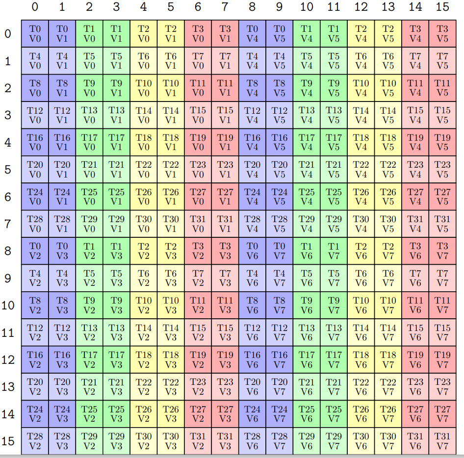
现在对于一个 thread 我们要获得其对应的 scale,这应该如何做到?对于 W scale 很简单,因为一个 cta tile 只有一个 scale,大家都是共享的。对于 X scale 则复杂一些,我们需要寻找这些元素所对应的 m index,即:他们是属于哪一行的。此时 layout algebra 就要大展身手了!hpc-ops 使用了 identity matrix + partition 来解决这个问题:
所谓 identity layout 就是将其输入映射到自身的 layout,这里的自身是一个 coordinate 而不是单纯的整数。这在之前介绍 tma 的时候有所介绍
layout = make_identity_layout((4,4))     # stride=(1@0,1@1)
layout(0, 1) = (0, 1)   # a coordinate tuple
所以当我们对 index 有所需求的时候,考虑 identity matrix 都会是不错的选择。hpc-ops 对 C matrix 构建了 identity layout,然后用相同的 partition 方法对齐进行划分,这样就得到了每一个元素的 coordiante
auto gI = make_identity_tensor(gC.shape());
auto tI = thr_mma.partition_C(gI);           // (V, M, N)
auto tCr = thr_mma.partition_fragment_C(gC); // (V, M, N)
如此一来,对于任意的 tCr 的坐标都会知晓,我们可以直接取 coord 的 0 index 即可
hpc-ops 还使用 retile_fragment 把线程中的数据 retile 成为我们熟悉的二维 mn 形状,然后再进行循环累加。其实有了第一点的铺垫,这个 trick 完全可以省略。不过我认为这个变换能更帮助我深入理解 partition & C layout,所以整理。在上面我们提到 partition 过后的 tensor layout 为 (V, M, N),这是一个 cute 当中非常常见且极其重要的一个形式,当我们使用 C layout partition 一个 tensor 时:
- V 代表了一种 Local view,即:一个 C layout 内部,单个 thread 所得到的 value
- M 代表了在 M-dim 重复的数量,即: C layout 在 M 维度上有 M 个
- N 代表了在 N-dim 重复的数量,即: C layout 在 N 维度上有 N 个
这就是 partition 的本质 zipped divide + compose:用一个 layout mn 去划分一个 tensor mn (zipped_divide),并通过 layout tv -> mn 最终获得每一个 thread 获得的 value (compose)。
回到我们的问题当中,我们需要把 tI 或者 tCr 从 (V, M, N) 转换到 (M, N) 上来,应该怎么做?我们势必要对前面的 V 维度做进一步的拆解。实际上这里的 V 维度还可拆解为 (frg_V, frg_M, frg_N) 三个维度。为何?直接看 mma trait 当中的 C layout
using CLayout_64xN   = Layout<Shape <Shape <  _4,_8, _4>,Shape < _2,_2,Int<N/8>>>,
                        Stride<Stride<_128,_1,_16>,Stride<_64,_8,   _512>>>;

using CLayout_64x8   = CLayout_64xN<  8>;
using CLayout_64x16  = CLayout_64xN< 16>;
...
using CLayout_64x256 = CLayout_64xN<256>;
C layout 的 V 维度就是 3 个维度 (2, 2, N/8),其对应了 (frg_V, frg_M, frg_N)。时刻记住 C layout 代表了 tv -> mn 映射,所以 frg_V 维度一定是在 N-dim 上连续的,因为其 stride = 64,而 C layout 所对应 M shape 始终为 64。好了我们现在就可以做 retile (or reshape)
(V, M, N) -> ((frg_V, frg_M, frg_N), M, N) -> ((frg_M, M), (frg_V, frg_N, N))
// (frg_M, M) -> contigous in M dim
// (frg_V, frg_N, N) -> contigous in N dim
最终形成了 ((frg_M, M), (frg_V, frg_N, N)) 的形式,我们把 M 和 N 维度连续的轴各自排到了一起,这就是 hpc-ops 当中的 retile_fragment 所做的事
注意:我们在之前提到 hpc-ops 在进行 GEMM 运算时是将 X 和 W 进行交换的,所以以上的分析在真实的代码当中,都需要进行交换
mainloop 伪代码
我们对着伪代码代码简单走读一下,对整个过程的实现有一个理解。注意这里使用了 hpc-ops 当中交换 mma AB 矩阵的技巧
// Scale tensor layout in shared memory
// SLayoutXS: (kStage, kTileS) with stride (kTileS, 1)
// SLayoutWS: (kStage, kTileS) with stride (kTileS, 1)
auto sAS = make_tensor(make_smem_ptr(shm_as), SLayoutAS{});
auto sBS = make_tensor(make_smem_ptr(shm_bs), SLayoutBS{});

// K-dimension accumulation loop
for (int itile_k = 0; itile_k < ntile_k; ++itile_k) {
    // wait for data load to complete
    wait_barrier(readable[ismem_read], phase);

    // Step 1: read wscale from shared memory
    // Note: itile_k % 4 to get the required wscale index
    float wscale = sBS(ismem_read, itile_k % 4);

    // Step 2: compute xscale * wscale to get intermediate scale tCS
    float tCS[kN];
#pragma unroll
    for (int in = 0; in < kN; in++) {
    tCS[in] = sAS(ismem_read, get<1>(tI_mn(0, in))) * wscale;
    }

    // Step 3: GMMA computation (without scale)
    tiled_mma.accumulate_ = GMMA::ScaleOut::Zero;
    for (int ik = 0; ik < size<2>(tAr); ++ik) {
    cute::gemm(tiled_mma, tBr, tAr, tCr);
    }

    // Step 4: dequantize using scale
    auto tDr_mn = retile_fragment(tDr);
#pragma unroll
    for (int in = 0; in < kN; in++) {
    float yscale = tCS[in];  // each N dimension has independent scale
#pragma unroll
    for (int im = 0; im < kM; im++) {
        tDr_mn(im, in) = tCr_mn(im, in) * yscale + tDr_mn(im, in);
    }
    }
}